SQL for Feature Extraction (Part 2)#

1. Preliminary Knowledge#

In the previous series of articles SQL for Feature Extraction (Part 1), we introduce the basic concepts and practical tools of feature engineering, as well as the basic feature processing script development based on a single table. In this article, we will introduce more complex and more powerful feature processing script development on multi-tables. At the same time, we will take the SQL syntax of OpenMLDB as an example for SQL-based feature engineering development. For more information about OpenMLDB, please visit GitHub repo of OpenMLDB, and the document website.

If you want to run the SQL in this tutorial, please follow the following two steps to prepare:

It is recommended to use the OpenMLDB docker image under Standalone Version. Refer to OpenMLDB Quick Start for the operation mode. If using the cluster version, please use the Offline mode (SET @@execute_mode='offline' ). The CLI tool of cluster version is only available under Offline mode and Online Preview mode. The Online Preview mode only can be used for simple data preview, so most of the SQL in the tutorial cannot run in this mode.
All data related to this tutorial and the import operation script can be downloaded here.

In this article, the data set consists of a main table (holding the labels) and other secondary tables. We still use the sample data of anti-fraud transactions in the previous article, including a main table: user transaction table (Table 1, t1) and a secondary table: merchant flow table (Table 2, t2). In the design of relational database, in order to avoid data redundancy and ensure data consistency, commonly, the data are stored in multiple tables according to design principles (database design paradigm). In feature engineering, in order to obtain enough effective information, data needs to be extracted from multiple tables. As a result, feature engineering needs to be carried out based on multiple tables.

Main Table: User Transaction Table, t1

Field	Type	Description
id	BIGINT	Sample ID, each sample has an unique ID
uid	STRING	User ID
mid	STRING	Merchant ID
cardno	STRING	Card Number
trans_time	TIMESTAMP	Transaction Time
trans_amt	DOUBLE	Transaction Amount
trans_type	STRING	Transaction Type
province	STRING	Province
city	STRING	City
label	BOOL	Sample label, true\|false

Table 2: Merchant Transaction Table, t2

Field	Type	Description
mid	STRING	Merchant ID
card	STRING	Card Number
purchase_time	TIMESTAMP	Purchase Time
purchase_amt	DOUBLE	Purchase Amount
purchase_type	STRING	Purchase Type: Cash, Credit Card

2. LAST JOIN#

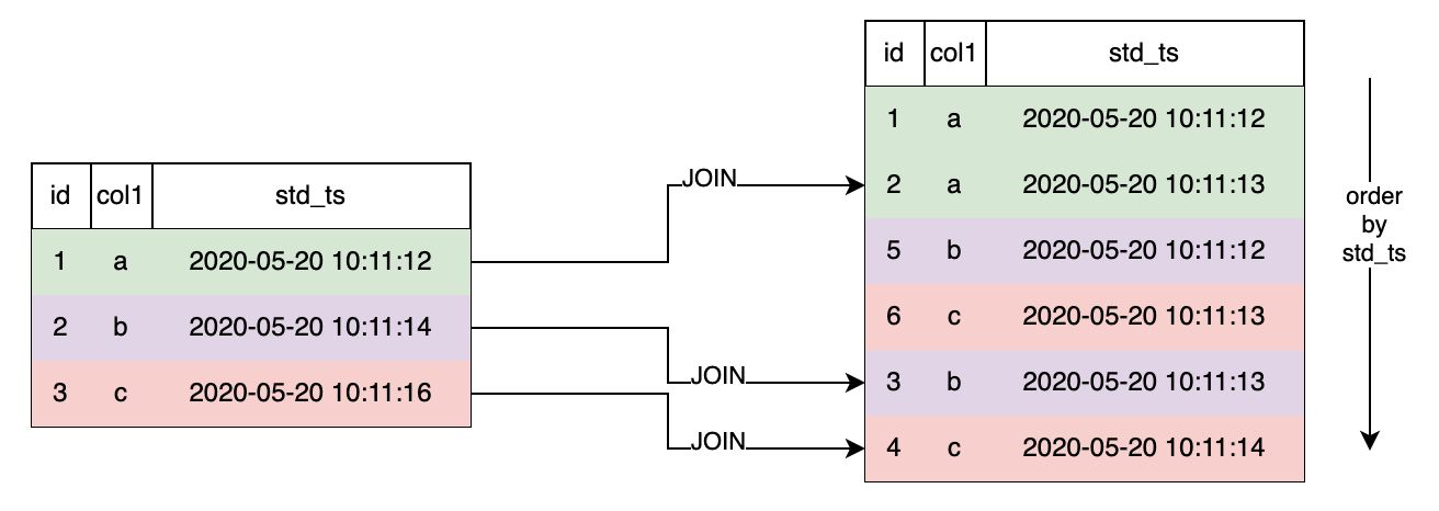
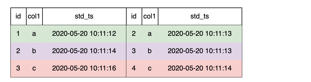
OpenMLDB supportsLAST JOIN as a variant of LEFT JOIN that is supported in the standard SQL. For each record in the left table, when there are multiple records matched from the right table, only one record will be output as the result. There are two types of LAST JOIN: ordered and non-ordered LAST JOIN. Let’s take a simple table as an example and assume that both the schemas of tables s1 and s2 are

(id int, col1 string, std_ts timestamp)

Then, we can do the following join operation:

SELECT * FROM s1 LAST JOIN s2 ORDER BY s2.std_ts ON s1.col1 = s2.col1;

As shown below, left table LAST JOIN right table with ORDER BY and right table is sorted by std_ts. Take the second row of the left table as an example. There are two matched rows in right table. After sorting by std_ts the last row 3, b, 2020-05-20 10:11:13 is selected.

3. Multi-Row Aggregation over Multiple Tables#

For aggregation over multiple tables, OpenMLDB extends the standard WINDOW syntax and adds WINDOW UNION syntax. WINDOW UNION supports combining multiple pieces of data from the secondary table to form a window on secondary table. Based on the time window, it is convenient to construct the multi-row aggregation feature of the secondary table. Similarly, two steps need to be completed to construct the multi-row aggregation feature of the secondary table:

Step 1: Define the time window over multiple tables.
Step 2: Construct the multi-row aggregation feature of the secondary table on the window constructed in Step 1.

3.1 Step 1: Define the Time Window over Multiple Tables#

Each row of the main table can concat multiple rows from the secondary table according to a certain column, and it is allowed to define the time interval or number interval of the data that can be combined. We use the WINDOW UNION to define the secondary table combining condition and interval range. To make it easier to understand, we call this kind of windows as secondary table combining windows.

The syntax of creating a secondary table combining window is defined as:

window window_name as (UNION other_table PARTITION BY key_col ORDER BY order_col ROWS_RANGE｜ROWS BETWEEN StartFrameBound AND EndFrameBound)

Among them, necessary elements include:

UNION other_table: other_table refers to the secondary table for WINDOW UNION. The primary and secondary tables’ schemas need to keep consistent. In most cases, the schema of the primary table and the secondary table are different. We can ensure the schema consistency of the primary and secondary tables involved in window calculation by column projection and default column configuration. Column projection can also remove useless columns and only do WINDOW UNION and aggregation on important columns.
PARTITION BY key_col: Indicates that main table and secondary table are combined according to column key_col.
ORDER BY order_col: Indicates that the secondary table is sorted in accordance withorder_col columns.
ROWS_RANGE BETWEEN StartFrameBound AND EndFrameBound: Represents the time interval of the secondary table combining window.
- StartFrameBound represents the upper bound of the window.
  - UNBOUNDED PRECEDING: There is no upper bound.
  - time_expression PRECEDING: If it is a time interval, you can define a time offset. For example, 30d preceding means that the upper bound of the window is 30 days before the time of the current row.
- EndFrameBound Represents the lower bound of the time window.
  - CURRENT ROW: The lower bound is current row.
  - time_expression PRECEDING: If it is a time interval, you can define a time offset, such as 1d PRECEDING. This indicates that the lower bound of the window is 1 day before the time of the current row.
ROWS BETWEEN StartFrameBound AND EndFrameBound: Represents the time interval of the secondary table combining window.
- StartFrameBound represents the upper bound of the window.
  - UNBOUNDED PRECEDING: There is no upper bound.
  - number PRECEDING: If it is a number interval, you can define the number of rows. For example, 100 PRECEDING indicates that the upper bound is 100 lines before the current row.
- EndFrameBound Represents the lower bound of the window.
  - CURRENT ROW: The lower bound is current row.
  - number PRECEDING: If it is a number interval, you can define the number of rows. For example, 1 PRECEDING indicates that the lower bound is 1 line before the current line.

Note

When configuring the window interval boundary, please note that:
- At present, OpenMLDB cannot support the time after the current row as the upper and lower bounds. For example, 1d FOLLOWING is not supported. In other words, we can only deal with the historical time window. This also basically meets most of the application scenarios of feature engineering.
- Lower bound time must be > = Upper bound time
- The row number of lower bound must be < = The row number of upper bound
INSTANCE_NOT_IN_WINDOW: It indicates that except for the current row, other data in the main table will not enter the window.
For more syntax and features, please refer to OpenMLDB WINDOW UNION Reference Manual.

Example#

Let’s see the usage of WINDOW UNION through specific examples.

For the user transaction table t1 mentioned above, we define a window over the secondary table, that is merchant flow table t2, based on mid. Because the schemas of t1 and t2 are different, we extract the same columns from t1 and t2 respectively. For non-existent columns, we set default values. Among them, mid column is used as the combining condition of two tables, so it must be included. Secondly, the timestamp column（trans_time in t1 and purchase_time in t2）contains timing information, which is also necessary when defining the time window. The remaining columns are filtered and retained as required according to the aggregation function.

The following SQL and images show how to extract necessary columns from t1 to generate t11.

(select id, mid, trans_time as purchase_time, 0.0 as purchase_amt, "" as purchase_type from t1) as t11

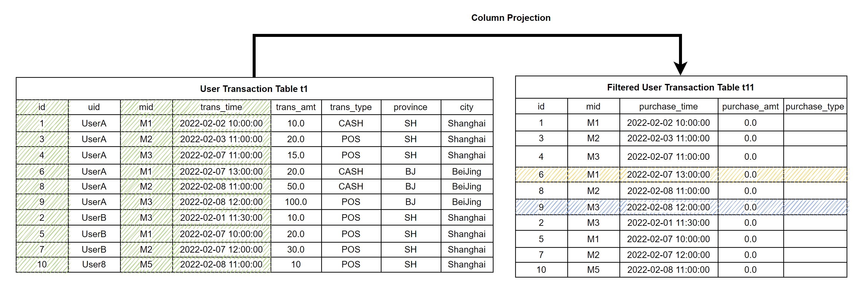
The following SQL extracts the necessary columns from t2 to generate t22.

(select 0L as id, mid, purchase_time, purchase_amt, purchase_type from t2) as t22

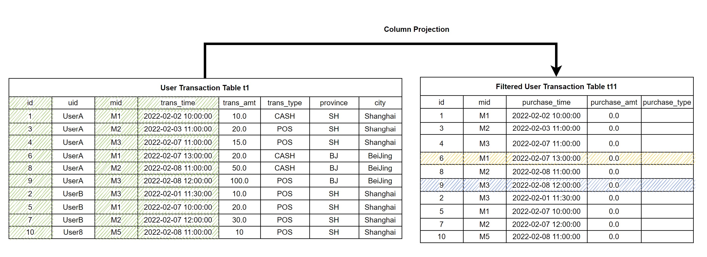
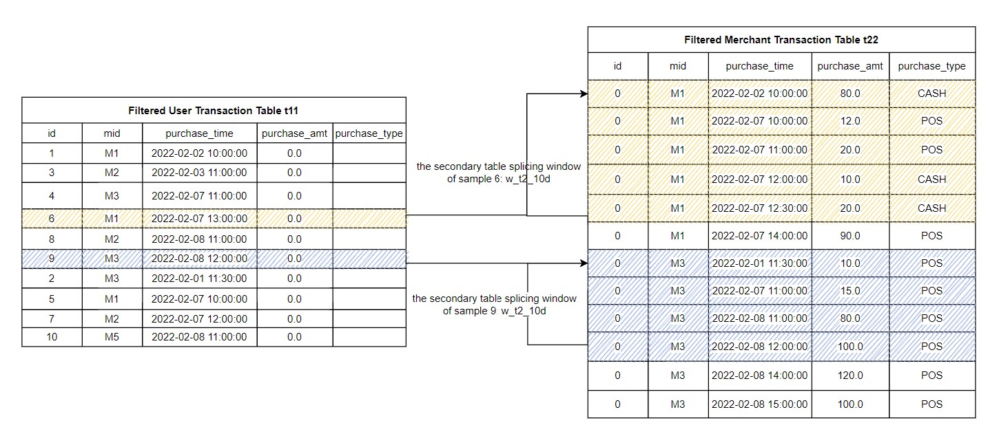
It can be seen that the newly generated t11 and t22 have the same schema, and they can perform logical union operation. However, in OpenMLDB, the WINDOW UNION is not really the same as the UNION operation in the traditional database, but to build the time window on the secondary table t22 for each row in t11. According to the merchant ID mid, we obtain the corresponding rows from t22 for each row in t11, and then sort them according to the consumption time (purchase_time) to construct the secondary table combining window. For example, we define a w_t2_10d window, which does not include the rows of the main table except the current row, but includes the data within ten days that is joint according to mid from the secondary table. The schematic is shown below. It can be seen that the yellow and blue shaded parts respectively represent the secondary table combining windows of sample 6 and sample 9.

The SQL script defining the above window is shown below (note that this is not a complete SQL):

(SELECT id, mid, trans_time as purchase_time, 0.0 as purchase_amt, "" as purchage_type FROM t1) as t11
window w_t2_10d as (
UNION (SELECT 0L as id, mid, purchase_time, purchase_amt, purchase_type FROM t2) as t22 
PARTITION BY mid ORDER BY purchase_time
ROWS_RANGE BETWEEN 10d PRECEDING AND 1 PRECEDING INSTANCE_NOT_IN_WINDOW)

3.2 Step 2: Build Multi-Row Aggregation Feature of Sub Table#

Apply the multi-row aggregation function on the created window to construct aggregation features on multi-rows of secondary table, so that the number of rows finally generated is the same as that of the main table. For example, we can construct features from the secondary table like: the total retail sales of merchants in the last 10 days w10d_merchant_purchase_amt_sum and the total consumption times of the merchant in the last 10 days w10d_merchant_purchase_count.

The following SQL constructs the multi-row aggregation feature based on the secondary table combining window defined in 3.1.

SELECT 
id, 
-- Total retail sales of sample merchants in the last 10 days
sum(purchase_amt) over w_t2_10d as w10d_merchant_purchase_amt_sum,
-- Transaction times of sample merchants in the last 10 days
count(purchase_amt) over w_t2_10d as w10d_merchant_purchase_count 
FROM   
(SELECT id, mid, trans_time as purchase_time, 0.0 as purchase_amt, "" as purchase_type FROM t1) as t11
window w_t2_10d as (
UNION (SELECT 0L as id, mid, purchase_time, purchase_amt, purchase_type FROM t2) as t22 
PARTITION BY mid ORDER BY purchase_time
ROWS_RANGE BETWEEN 10d PRECEDING AND 1 PRECEDING INSTANCE_NOT_IN_WINDOW)

4. Feature Group Construction#

Generally speaking, a complete feature extraction script will extract dozens or even hundreds of features. We can divide these features into several groups according to the feature type, the table and window associated with the feature, and then put each group of features into different SQL sub queries. Finally, the results of these sub queries are combined according to the main table ID. In this section, we will continue the previous examples to demonstrate how to form a feature wide table combining various features.

First, we divide the features into 3 groups:

Feature Group	Description
1	Single row features of users table (primary table) and merchants table (secondary table)
2	Window aggregation features of users table (main table) in the last 30 days and the last 7 days
3	Aggregation features of merchants table (secondary table) in the last 30 days

Then, we use OpenMLDB SQL to create the features of the same group in one sub query:

Feature Group 1

  -- Main table single line features
  SELECT 
  -- Column direct extraction
  id, uid, trans_type, 
  -- Single line time characteristics：day of week
  dayofweek(trans_time) as f_trans_day_of_week, 
  -- Time characteristics of single line: Transaction day
  day(trans_time) as f_trans_day, 
  -- Single line time characteristics: Transaction hours
  hour(trans_time) as f_trans_hour, 
  -- Single line time characteristics: Transaction minutes
  minute(trans_time),
  -- Mathematical characteristics of single line: The transaction amount is rounded up and then taken as logarithm
  log(ceiling(trans_amt)) as f_trans_amt_log,
  -- Single line string feature: The first four digits of card number
  substr(cardno, 1, 4),
  -- Secondary table features
  t2.purchase_time as f_purchase_time, 
  t2.purchase_amt as f_purchase_amt, 
  t2.purchase_type as f_purchase_type
  
  FROM t1 LAST JOIN t2 ORDER BY t2.purchase_time ON t1.mid = t2.mid

Feature Group 2

  -- Main table window features
  SELECT 
  id as out2id,
  -- Total POS transaction amount in the last 30 days
  sum_where(trans_amt, trans_type = "POS") over w30d as w30d_sum_pos_trans_amt,
  -- Maximum POS transaction amount in the last 30 days
  max_where(trans_amt, trans_type = "POS") over w30d as w30d_max_pos_trans_amt,
  -- Average single POS transaction amount in the last 30 days
  avg_where(trans_amt, trans_type = "POS") over w30d as w30d_avg_pos_trans_amt,
  -- Total number of POS transactions in the last 30 days
  count_where(trans_amt, trans_type = "POS") over w30d as w30d_count_pos_trans_amt,
  
  -- Total transaction amount in the last week
  sum(trans_amt) over w7d as w7d_sum_trans_amt,
  -- Total number of transactions in the last week
  count(trans_amt) over w7d as w7d_count_trans_amt,
  from t1
  -- Windows in the last 30 days
  window w30d as (PARTITION BY uid ORDER BY trans_time ROWS_RANGE BETWEEN 30d PRECEDING AND CURRENT ROW),
  -- Last week's window
  w7d as (PARTITION BY uid ORDER BY trans_time ROWS_RANGE BETWEEN 7d PRECEDING AND CURRENT ROW)

Feature Group 3

-- Side table aggregation feature
  SELECT 
  id as out3id,
  -- Total retail sales of sample merchants in the last week
  sum(purchase_amt) over w7d_merchant as w7d_merchant_purchase_amt_sum,
  -- Transaction times of sample merchants in the last week
  count(purchase_amt) over w7d_merchant as w7d_merchant_purchase_count,
  -- Main table merchant's flow in the last week
  FROM (select id, mid, cardno as card, trans_time as purchase_time, 0.0 as purchase_amt, "" as purchase_type from t1) as t11
   window w7d_merchant as (UNION (select 0L as id, mid, card, purchase_time, purchase_amt, purchase_type from t2) as t22 PARTITION BY mid ORDER BY purchase_time ROWS_RANGE BETWEEN 30d PRECEDING AND 1 PRECEDING INSTANCE_NOT_IN_WINDOW)

Finally, the three groups of features are combined according to the main table ID:

SELECT * FROM 
-- Feature group 1
(
  -- Main table single line features
  SELECT 
  -- Column direct extraction
  id, uid, trans_type, 
  -- Single line time characteristics：Day of week
  dayofweek(trans_time) as f_trans_day_of_week, 
  -- Time characteristics of single line: Transaction day
  day(trans_time) as f_trans_day, 
  -- Single line time characteristics: Transaction hours
  hour(trans_time) as f_trans_hour, 
  -- Single line time characteristics: Transaction minutes
  minute(trans_time),
  -- Mathematical characteristics of single line: The transaction amount is rounded up and then taken as logarithm
  log(ceiling(trans_amt)) as f_trans_amt_log,
  -- Single line string feature: The first four digits of card number
  substr(cardno, 1, 4),
  
  -- Secondary table features
  t2.purchase_time as f_purchase_time, 
  t2.purchase_amt as f_purchase_amt, 
  t2.purchase_type as f_purchase_type
  
  FROM t1 LAST JOIN t2 ORDER BY t2.purchase_time ON t1.mid = t2.mid
) as out1 LAST JOIN 
-- Feature group 2
(
  -- Main table window features
  SELECT 
  id as out2id,
  -- Total POS transaction amount in the last 30 days
  sum_where(trans_amt, trans_type = "POS") over w30d as w30d_sum_pos_trans_amt,
  -- Maximum POS transaction amount in the last 30 days
  max_where(trans_amt, trans_type = "POS") over w30d as w30d_max_pos_trans_amt,
  -- Average single POS transaction amount in the last 30 days
  avg_where(trans_amt, trans_type = "POS") over w30d as w30d_avg_pos_trans_amt,
  -- Total number of POS transactions in the last 30 days
  count_where(trans_amt, trans_type = "POS") over w30d as w30d_count_pos_trans_amt,
  
  -- Total transaction amount in the last week
  sum(trans_amt) over w7d as w7d_sum_trans_amt,
  -- Total number of transactions in the last week
  count(trans_amt) over w7d as w7d_count_trans_amt 
  from t1
  -- Windows in the last 30 days
  window w30d as (PARTITION BY uid ORDER BY trans_time ROWS_RANGE BETWEEN 30d PRECEDING AND CURRENT ROW),
  -- Last week's window
  w7d as (PARTITION BY uid ORDER BY trans_time ROWS_RANGE BETWEEN 7d PRECEDING AND CURRENT ROW)
) as out2 ON out1.id = out2.out2id LAST JOIN
-- Feature group 3
(
   -- Side table aggregation feature
   SELECT
   id as out3id,
   -- Total retail sales of sample merchants in the last week
   sum(purchase_amt) over w7d_merchant as w7d_merchant_purchase_amt_sum,
   -- Transaction times of sample merchants in the last week
   count(purchase_amt) over w7d_merchant as w7d_merchant_purchase_count
   -- Main table merchant's flow in the last week
   FROM (select id, mid, cardno as card, trans_time as purchase_time, 0.0 as purchase_amt, "" as purchase_type from t1) as t11
   window w7d_merchant as (UNION (select 0L as id, mid, card, purchase_time, purchase_amt, purchase_type from t2) as t22 PARTITION BY mid ORDER BY purchase_time ROWS_RANGE BETWEEN 30d PRECEDING AND 1 PRECEDING INSTANCE_NOT_IN_WINDOW)
) as out3 ON out1.id = out3.out3id;

SQL for Feature Extraction (Part 2)

Contents