Standalone Usage Process
Contents
Standalone Usage Process#
Preparation#
This article provides a guide on developing and deploying with OpenMLDB CLI. To begin, you need to download the sample data and start the OpenMLDB CLI. It is recommended to utilize a prepared Docker image for a faster start.
Docker (minimum version: 18.03)
Pull Mirror Image#
Execute the following command to fetch the OpenMLDB image and initiate a Docker container:
docker run -it 4pdosc/openmldb:0.9.2 bash
Upon successful container launch, all subsequent commands in this tutorial will assume execution within the container.
If you require external access to the OpenMLDB server within the container, please consult CLI/SDK-Container onebox.
Download Sample Data#
Execute the following command to download the sample data for the subsequent procedures:
curl https://openmldb.ai/demo/data.csv --output /work/taxi-trip/data/data.csv
Start Server and Client#
Start the standalone OpenMLDB server
./init.sh standalone
Start the standalone OpenMLDB CLI client
cd taxi-trip
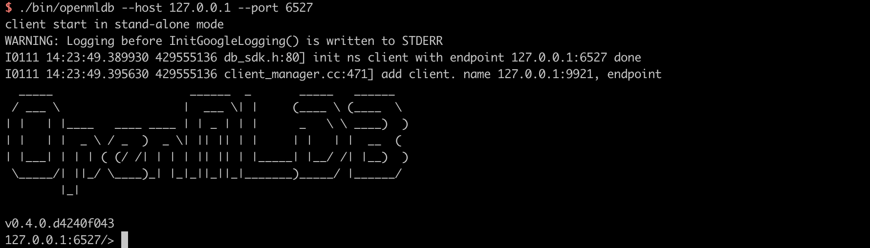
/work/openmldb/bin/openmldb --host 127.0.0.1 --port 6527
The following image displays the screen after the correct execution of commands within Docker, indicating a successful launch of OpenMLDB CLI:
Usage#
The workflow for the standalone version of OpenMLDB typically comprises five stages:
Database and table creation.
Data preparation.
Offline feature computation.
SQL Deployment.
Real-time feature computation.
Unless otherwise specified, the following commands are executed by default within the standalone version of the OpenMLDB CLI.
Step 1: Database and Table Creation#
CREATE DATABASE demo_db;
USE demo_db;
CREATE TABLE demo_table1(c1 string, c2 int, c3 bigint, c4 float, c5 double, c6 timestamp, c7 date);
Step 2: Data Preparation#
Import the sample data previously downloaded as training data for both offline and online feature computations.
It’s important to note that in the standalone version, table data is not segregated for offline and online usage. Thus, the same table is employed for both offline and online feature computations. Alternatively, you have the option to manually import different data for offline and online use, resulting in the creation of two separate tables. However, for simplicity, this tutorial employs the same data for both offline and online computations in the standalone version.
Execute the following command to import data:
LOAD DATA INFILE 'data/data.csv' INTO TABLE demo_table1;
Preview data:
SELECT * FROM demo_table1 LIMIT 10;

 ----- ---- ---- ---------- ----------- --------------- ------------

  c1    c2   c3   c4         c5          c6              c7

 ----- ---- ---- ---------- ----------- --------------- ------------

  aaa   12   22   2.200000   12.300000   1636097390000   2021-08-19

  aaa   11   22   1.200000   11.300000   1636097290000   2021-07-20

  dd    18   22   8.200000   18.300000   1636097990000   2021-06-20

  aa    13   22   3.200000   13.300000   1636097490000   2021-05-20

  cc    17   22   7.200000   17.300000   1636097890000   2021-05-26

  ff    20   22   9.200000   19.300000   1636098000000   2021-01-10

  bb    16   22   6.200000   16.300000   1636097790000   2021-05-20

  bb    15   22   5.200000   15.300000   1636097690000   2021-03-21

  bb    14   22   4.200000   14.300000   1636097590000   2021-09-23

  ee    19   22   9.200000   19.300000   1636097000000   2021-01-10

 ----- ---- ---- ---------- ----------- --------------- ------------
Step 3: Offline Feature Computation#
Execute SQL commands to extract features and store the resulting features in a file for subsequent model training.
SELECT c1, c2, sum(c3) OVER w1 AS w1_c3_sum FROM demo_table1 WINDOW w1 AS (PARTITION BY demo_table1.c1 ORDER BY demo_table1.c6 ROWS BETWEEN 2 PRECEDING AND CURRENT ROW) INTO OUTFILE '/tmp/feature.csv';
Step 4: SQL Deployment#
Deploy the SQL script developed offline for online feature computation. It’s crucial to ensure that the deployed SQL is the same as the corresponding offline SQL.
DEPLOY demo_data_service SELECT c1, c2, sum(c3) OVER w1 AS w1_c3_sum FROM demo_table1 WINDOW w1 AS (PARTITION BY demo_table1.c1 ORDER BY demo_table1.c6 ROWS BETWEEN 2 PRECEDING AND CURRENT ROW);
Once the deployment is complete, you can access the deployed SQL using the SHOW DEPLOYMENTS command.
SHOW DEPLOYMENTS;

 --------- -------------------

  DB        Deployment

 --------- -------------------

  demo_db   demo_data_service

 --------- -------------------

1 row in set
Note
In this standalone version of the tutorial, the same dataset is utilized for both offline and online feature computations. If a user prefers to work with a different dataset, they must import the new dataset prior to deployment. During deployment, the tables associated with the new dataset should be used.
Exit CLI#
quit;
At this stage, all development and deployment tasks using OpenMLDB CLI have been completed, and we return to the command line.
Step 5: Real-Time Feature Computation#
Real-time online services can be accessed through the following web APIs:
http://127.0.0.1:8080/dbs/demo_db/deployments/demo_data_service
\___________/ \____/ \_____________/
| | |
APIServer Address Database Name Deployment Name
Now, the real-time system is ready to accept input data in JSON format. Here’s an example: you can place a row of data into the designated input field.
curl http://127.0.0.1:8080/dbs/demo_db/deployments/demo_data_service -X POST -d'{"input": [["aaa", 11, 22, 1.2, 1.3, 1635247427000, "2021-05-20"]]}'
The expected return results for this query are as follows (the computed features will be stored in the data field):
{"code":0,"msg":"ok","data":{"data":[["aaa",11,22]]}}
Explanation:
The API server can process requests and support batch requests. Arrays are supported via the
inputfield, with each line of input processed individually. For detailed parameter formats, please refer to the REST API documentation.To understand the results of real-time feature computation requests, please refer to the Description of Real-Time Feature Computation Results.