OpenMLDB Quickstart
Contents
OpenMLDB Quickstart#
Basic Concepts#
The main use case of OpenMLDB is as a real-time feature platform for machine learning. The basic usage process is shown in the following diagram:
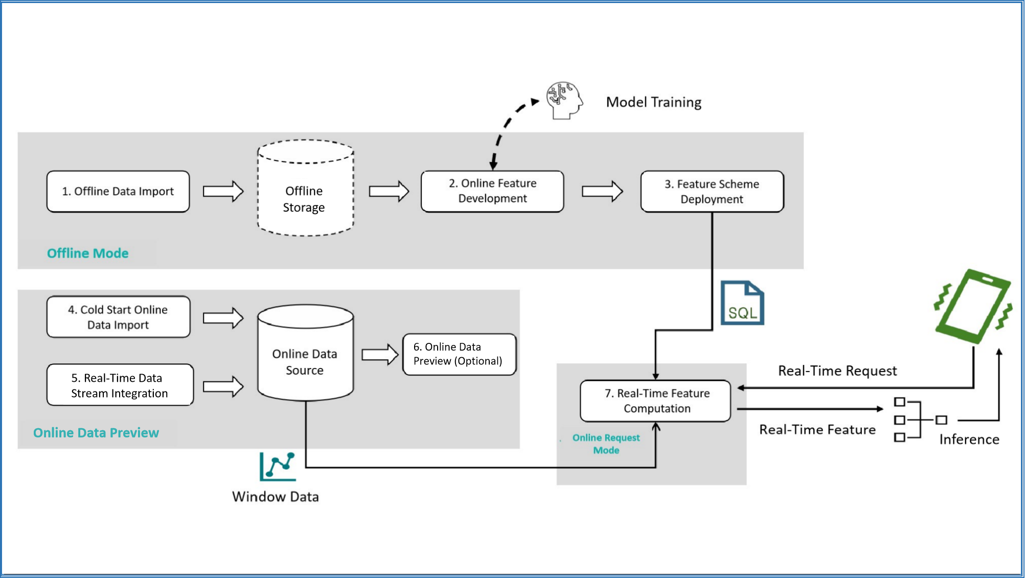
As shown, OpenMLDB covers the feature computing process in machine learning, from offline development to real-time serving online, providing a complete process. Please refer to the documentation for The Usage Process and Execution Mode in detail. This article will demonstrate a quickstart step by step, showing the process for basic usage.
Preparation#
This sample program is developed and deployed based on OpenMLDB CLI, so you need to download the sample data and start OpenMLDB CLI first. It is recommended to use Docker image for a quick experience (Note: due to some known issues of Docker on macOS, the sample program in this article may encounter problems on macOS. It is recommended to run it on Linux or Windows).
Docker Version: >= 18.03
Pull the Image#
Execute the following command in the command line to pull the OpenMLDB image and start the Docker container:
docker run -it 4pdosc/openmldb:0.9.2 bash
Note
After successfully starting the container, all subsequent commands in this tutorial are executed inside the container by default. If you need to access the OpenMLDB server inside the container from outside the container, please refer to the CLI/SDK-container onebox documentation.
Start the Server and Client#
Start the OpenMLDB server:
/work/init.sh
Start the OpenMLDB CLI client:
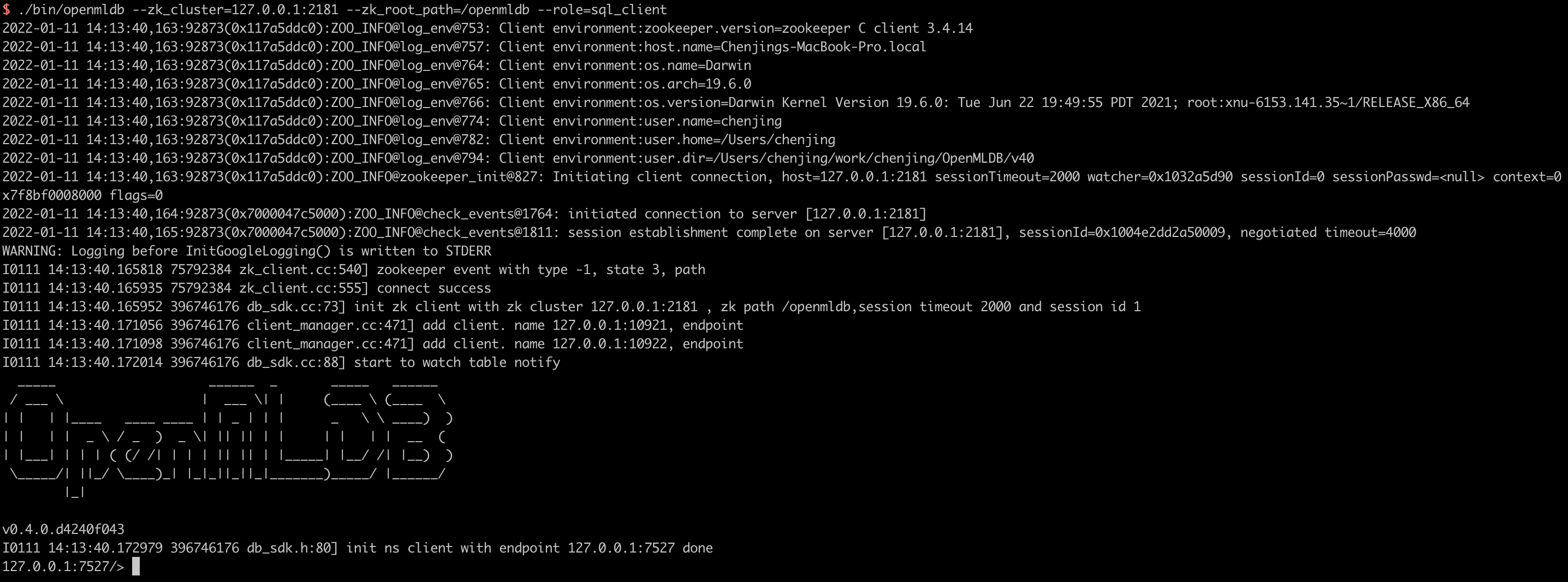
/work/openmldb/bin/openmldb --zk_cluster=127.0.0.1:2181 --zk_root_path=/openmldb --role=sql_client
# or script
/work/openmldb/sbin/openmldb-cli.sh
Successful started OpenMLDB CLI will look as shown in the following figure:
If you need to modify the configuration of the OpenMLDB cluster, and the /work/init.sh uses the sbin one-click deployment method, please refer to the One-Click Deployment for specific instructions.
OpenMLDB Process#
Referring to the core concepts, the process of using OpenMLDB generally includes six steps: create database and table, import offline data, compute offline feature, deploy SQL plan, import online data, and online real-time feature compute.
Note
Unless otherwise specified, the commands demonstrated below are executed by default in OpenMLDB CLI.
Step 1: Create Database and Table#
Create demo_db and table demo_table1:
-- OpenMLDB CLI
CREATE DATABASE demo_db;
USE demo_db;
CREATE TABLE demo_table1(c1 string, c2 int, c3 bigint, c4 float, c5 double, c6 timestamp, c7 date);
Step 2: Import Offline Data#
Switch to the offline execution mode, and import the sample data as offline data for offline feature calculation.
-- OpenMLDB CLI
USE demo_db;
SET @@execute_mode='offline';
LOAD DATA INFILE 'file:///work/taxi-trip/data/data.parquet' INTO TABLE demo_table1 options(format='parquet', mode='append');
Note that the LOAD DATA command is an asynchronous command by default. You can use the following command to check the task status and detailed logs:
To show the list of submitted tasks: SHOW JOBS
To show the detailed information of a task: SHOW JOB job_id (job_id can be obtained from the SHOW JOBS command)
To show the task logs: SHOW JOBLOG job_id
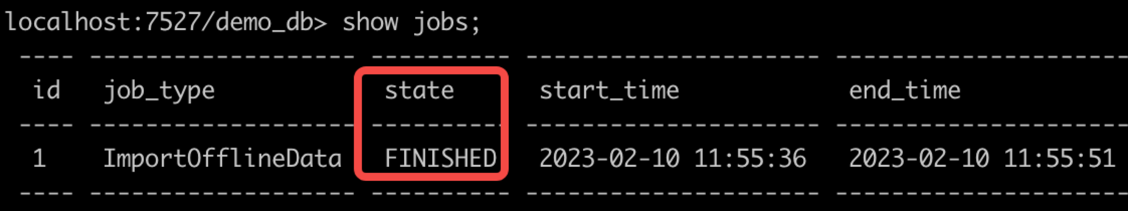
Here, we use SHOW JOBS to check the task status. Please wait for the task to be successfully completed ( state changes to FINISHED), and then proceed to the next step.
After the task is completed, if you wish to preview the data, you can execute the SELECT * FROM demo_table1 statement in synchronous mode by setting SET @@sync_job=true. However, this approach has certain limitations, which are detailed in the Offline Command Synchronous Mode section.
In the default asynchronous mode, executing SELECT * FROM demo_table1 will initiate an asynchronous task, and the results will be stored in the log files of the Spark job, making them less convenient to access. If TaskManager is in local mode, you can use SHOW JOBLOG <id> to view the query print results in the stdout section.
The most reliable way to access the data is to use the SELECT INTO command to export the data to a specified directory or directly examine the storage location after importing it.
Note
OpenMLDB also supports importing offline data through linked soft copies, without the need for hard data copying. Please refer to the parameter deep_copy in the LOAD DATA INFILE Documentation for more information.
Step 3: Compute Offline Feature#
Assuming that we have determined the SQL script (SELECT statement) to be used for feature computation, we can use the following command for offline feature computation:
-- OpenMLDB CLI
USE demo_db;
SET @@execute_mode='offline';
SET @@sync_job=false;
SELECT c1, c2, sum(c3) OVER w1 AS w1_c3_sum FROM demo_table1 WINDOW w1 AS (PARTITION BY demo_table1.c1 ORDER BY demo_table1.c6 ROWS BETWEEN 2 PRECEDING AND CURRENT ROW) INTO OUTFILE '/tmp/feature_data' OPTIONS(mode='overwrite');
The SELECT INTO command is an asynchronous task. Use the SHOW JOBS command to check the task running status. Please wait for the task to complete successfully (state changes to FINISHED) before proceeding to the next step.
Note:
Similar to the
LOAD DATAcommand, theSELECTcommand also runs asynchronously by default in offline mode.The
SELECTstatement is used to perform SQL-based feature extraction and store the generated features in the directory specified by theOUTFILEparameter asfeature_data, which can be used for subsequent machine learning model training.
Step 4: Deploy SQL plan#
Switch to online preview mode, and deploy the explored SQL plan to online. The SQL plan is named demo_data_service, and the online SQL used for feature extraction needs to be consistent with the corresponding offline feature calculation SQL.
-- OpenMLDB CLI
SET @@execute_mode='online';
USE demo_db;
DEPLOY demo_data_service SELECT c1, c2, sum(c3) OVER w1 AS w1_c3_sum FROM demo_table1 WINDOW w1 AS (PARTITION BY demo_table1.c1 ORDER BY demo_table1.c6 ROWS BETWEEN 2 PRECEDING AND CURRENT ROW);
After the deployment, you can use the command SHOW DEPLOYMENTS to view the deployed SQL.
Step 5: Import Online Data#
Import the downloaded sample data as online data for online feature computation in online mode.
-- OpenMLDB CLI
USE demo_db;
SET @@execute_mode='online';
LOAD DATA INFILE 'file:///work/taxi-trip/data/data.parquet' INTO TABLE demo_table1 options(format='parquet', header=true, mode='append');
LOAD DATA is an asynchronous command by default, you can use offline task management commands such as SHOW JOBS to check the progress. Please wait for the task to complete successfully (state changes to FINISHED) before proceeding to the next step.
After the task is completed, you can preview the online data:
-- OpenMLDB CLI
USE demo_db;
SET @@execute_mode='online';
SELECT * FROM demo_table1 LIMIT 10;
Note that currently, it is required to successfully deploy the SQL plan before importing online data; importing online data before deployment may cause deployment errors.
Note
The tutorial skips the step of real-time data access after importing data. In practical scenarios, as time progresses, the latest real-time data needs to be updated in the online database. This can be achieved through the OpenMLDB SDK or online data source connectors such as Kafka, Pulsar, etc.
Step 6: Online Real-Time Feature Computing#
The development and deployment work is completed. Next, you can make real-time feature calculation requests in real-time request mode. First, exit OpenMLDB CLI and return to the command line of the operating system.
-- OpenMLDB CLI
quit;
According to the default deployment configuration, the http port for APIServer is 9080. Real-time online services can be provided through the following Web API:
http://127.0.0.1:9080/dbs/demo_db/deployments/demo_data_service
        \___________/      \____/              \_____________/
              |               |                        |
      APIServerAddress  Database Name           Deployment Name
Real-time requests accept input data in JSON format. Here are two examples: putting data in the input field of the request.
Example 1:
curl http://127.0.0.1:9080/dbs/demo_db/deployments/demo_data_service -X POST -d'{"input": [["aaa", 11, 22, 1.2, 1.3, 1635247427000, "2021-05-20"]]}'
Expected query result (the calculated features are stored in the data field):
{"code":0,"msg":"ok","data":{"data":[["aaa",11,22]]}}
Example 2:
curl http://127.0.0.1:9080/dbs/demo_db/deployments/demo_data_service -X POST -d'{"input": [["aaa", 11, 22, 1.2, 1.3, 1637000000000, "2021-11-16"]]}'
Expected query result:
{"code":0,"msg":"ok","data":{"data":[["aaa",11,66]]}}
Explanation of Real-Time Feature Computing Results#
The SQL execution for online real-time requests is different from batch processing mode. The request mode only performs SQL calculations on the data of the request row. In the previous example, it is the input of the POST request that serves as the request row. The specific process is as follows: Assuming that this row of data exists in the table demo_table1, and the following feature calculation SQL is executed on it:
SELECT c1, c2, sum(c3) OVER w1 AS w1_c3_sum FROM demo_table1 WINDOW w1 AS (PARTITION BY demo_table1.c1 ORDER BY demo_table1.c6 ROWS BETWEEN 2 PRECEDING AND CURRENT ROW);
The Calculation Logic for Example 1 is as Follows:
Filter rows in column c1 with the value “aaa” based on the
PARTITION BYpartition of the request row and window, and sort them in ascending order by column c6. Therefore, in theory, the intermediate data table sorted by partition should be as follows. The request row is the first row after sorting.
----- ---- ---- ---------- ----------- --------------- ------------
c1    c2   c3   c4         c5          c6              c7
----- ---- ---- ---------- ----------- --------------- ------------
aaa   11   22   1.2        1.3         1635247427000   2021-05-20
aaa   11   22   1.200000   11.300000   1636097290000   1970-01-01
aaa   12   22   2.200000   12.300000   1636097890000   1970-01-01
----- ---- ---- ---------- ----------- --------------- ------------
The window range is
2 PRECEDING AND CURRENT ROW. In the above table, when the actual window is extracted, the request row is the smallest row with no preceding 2 rows. Therefore the window only contains the request row.For window aggregation, the sum of column c3 for the data within the window (only one row) is calculated, resulting in 22. Therefore, the output result is:
----- ---- -----------
c1    c2   w1_c3_sum
----- ---- -----------
aaa   11      22
----- ---- -----------
The Calculation Logic for Example 2 is as Follows:
According to the partition of the request line and window by
PARTITION BY, select the rows where column c1 is “aaa” and sort them in ascending order by column c6. Therefore, theoretically, the intermediate data table after partition and sorting should be as shown in the table below. The request row is the last row after sorting.
----- ---- ---- ---------- ----------- --------------- ------------
c1    c2   c3   c4         c5          c6              c7
----- ---- ---- ---------- ----------- --------------- ------------
aaa   11   22   1.200000   11.300000   1636097290000   1970-01-01
aaa   12   22   2.200000   12.300000   1636097890000   1970-01-01
aaa   11   22   1.2        1.3         1637000000000   2021-11-16
----- ---- ---- ---------- ----------- --------------- ------------
The window range is
2 PRECEDING AND CURRENT ROW. When the actual window is extracted from the above table, the two preceding 2 rows of the request row exist, together with the current row. Therefore, there are three rows of data in the window.For window aggregation, the sum of column c3 for the data within the window (three rows) is calculated, resulting in 22 + 22 + 22 = 66. Therefore, the output result is:
----- ---- -----------
c1    c2   w1_c3_sum
----- ---- -----------
aaa   11      66
----- ---- -----------