Based on OpenMLDB v0.4.0 for a Fast Build Full Online Process AI Application - OpenMLDB: An Open-Source Machine Learning Database

This article is based on Dihao Chen’s speech in "OpenMLDB Meetup No.1".

Based on OpenMLDB v0.4.0 for a Fast Build Full Online Process AI Application

At the beginning of the project, OpenMLDB has many performance optimizations including JIT optimization based on LLVM, which can optimize the corresponding code generation through LLVM for different CPU architectures, Linux servers or MAC servers. Even the latest ARM architecture Apple Computer Based on M1 can make OpenMLDB optimize for this scenario.

As mentioned earlier, in some scenarios, OpenMLDB can improve the performance 10 times or even more than 10 times than in Spark. In fact, we also benefit from a lot of code optimization for Spark including window tilt optimization, window parallel optimization and so on, which it is not supported by open-source Spark. We even transformed the Spark source code to realize this customized performance optimization for AI scenarios.

OpenMLDB is also optimized in storage. Traditional database services are mostly based on files. This storage based on b+ tree data structure is still not suitable for high-performance online AI applications and may also need to be optimized according to timing characteristics. We have implemented a multi-level jump table data structure for partition keys and sorting keyboards which can further improve the reading and writing performance of OpenMLDB on the timing data.

Recently, we have officially released the version 0.4.0 of OpenMLDB. This version also has many performance and function optimizations. Therefore, this article will introduce some new features of the latest version of OpenMLDB 0.4.0 and how to quickly build a full process online AI application based on this new version.

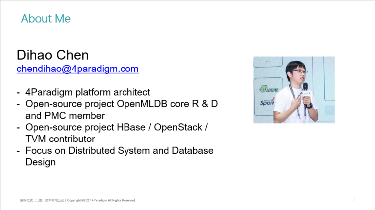
First of all, I'd like to make a brief self-introduction. My name is Dihao Chen. At present, I work as a platform architect in the 4Paradigm. I'm a core R & D and PMC member of the OpenMLDB project. I participated in the development of Over Distributed Storage HBase and Distributed Infrastructure OpenStack project. I'm a contributor to the TVM framework commonly used in machine learning. Currently, my main focus is on the Design of Distributed Systems and Databases.

P3：

Today, I will introduce you to three aspects:

New Features of the Whole Process of OpenMLDB 0.4.0
Quick Start of OpenMLDB 0.4.0 Stand-alone Version and Cluster Version
Teach you How to Use OpenMLDB to Quickly Build a Full Process Online AI Application

[01 | Introduction to New Features in the Whole Process of OpenMLDB 0.4.0]

OpenMLDB 0.4.0 New Features in the Whole Process 1 | Online and Offline Unified Storage

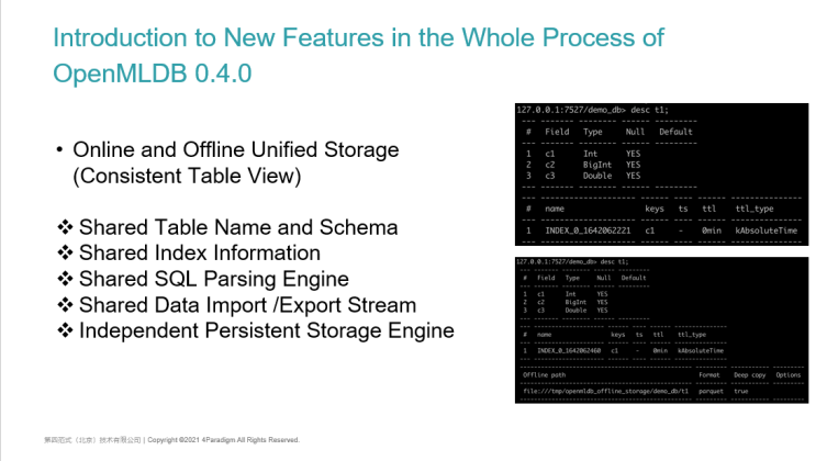
The first new feature is that the online storage and offline storage of OpenMLDB are unified (i.e., the view of the consistent table). In the upper right corner is our old version of table information. Through the SQL describe statement, you can see the name of the table T1, its schema information, how many columns it contains and the type in each column. Then, it follows by its index information.

In 0.4.0, we have added a unified table view which is to unify offline storage and online storage. In the lower right corner, an offline table information is added under the definition of an ordinary table. The information will include some attributes such as offline storage path and offline storage data format to see whether it is deep copy or not.

Unified storage is also a design rarely seen in databases in the industry. It enables offline tables and online tables to share a set of table names and schemes, a set of index information, and a SQL parsing engine. We use the SQL parsing engine implemented in C++ to compile SQL, and then share the same data import and export stream. In other words, both offline tables and online tables can use the same SQL statement for data import and export. The only difference between them is that offline and online tables have independent persistent storage respectively. The online storage we just mentioned is a full external memory high-performance multi-level hop table storage. Offline, we support local file storage and distributed storage such as HDFS to meet the needs of different offline and online scenarios.

OpenMLDB 0.4.0 New Features in the Whole Process 2 | High Availability Offline Task Management

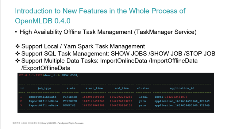
The second new feature is the addition of a highly available offline task management service called TaskManager Service,

The highly available offline task management service supports Spark task management on local or Yarn clusters and supports the use of SQL for task management such as SHOW JOBS, SHOW JOB, STOP JOB, etc. which are realized by expanding SQL syntax. It supports a variety of data tasks including importing online data, importing offline data, and exporting offline data.

OpenMLDB 0.4.0 New Features in the Whole Process 3 | End-to-end AI Workflow

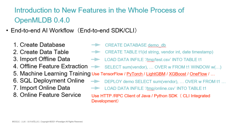
The third important feature is that it implements a real end-to-end AI workflow which can be used based on SDK or CLI command line.

The list on the left is the eight steps we are taking in the implementation of end-to-end AI applications. They are Creating a Database, Creating a Database Table, Importing Offline Data, Extracting Offline Features, and then Using the Machine Learning framework for model Training, Deploying SQL Online, Importing Online Data, and Online Feature Services.

From step 1 to step 8, almost every step can be implemented through the SDK or command line of OpenMLDB:

Use standard SQL statements to create databases and database tables which is supported by standard SQL
Like importing offline data, some SQL dialects can also be supported. For example, SQL server or MySQL can support a similar syntax of Load Data in File (i.e., Importing data from a file into a table)

We also support offline and online data import as well as offline feature extraction. As described earlier, our feature engineering uses the extended SQL language. We integrate the submission function of offline SQL tasks in the command line. You can execute a standard SQL on the command line such as the select sum statement here. However, because it is an offline task, after submitting a task with SQL, it will be submitted to a distributed computing cluster such as Yarn cluster, and then follow by doing the distributed offline feature engineering.

For Step 5 Machine Learning Model Training:

We support external machine learning training frameworks such as TensorFlow, PyTorch, LightGBM, XGBoost or OneFlow
Because we generate standard sample data formats, such as CSV, LIBSVM or TFRecords, users can use TensorFlow and other frameworks for model training
These frameworks can also be submitted to local, yarn cluster, k8s cluster, etc. for distributed training
It supports acceleration using GPU and other hardware and is fully compatible with our feature database OpenMLDB.

After the model training, that is when our SQL features can be online, then, we can directly execute a Deploy command and connect with the SQL that needs to be online This is when our online feature service is ready to be online. This is also achieved through SQL expansion.

To continue, the online service needs to inject some historical timing features into it which we call it the feature impoundment. Some historical data of users can also be completed by using the SQL statement of Load Data.

In the future, we can use the Java SDK, the Python SDK, or the internal HTTP service to complete the request. We will also integrate this function into CLI to realize the integration of end-to-end AI workflow of the whole process on the command line.

[02 | OpenMLDB 0.4.0 Stand-alone /Cluster Version Quick Start]

After introducing the new whole process features of 0.4.0, let's quickly start the functions of stand-alone version and cluster version of 0.4.0.

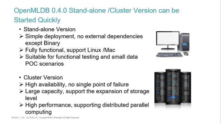
First, the difference between stand-alone version and cluster version is:

The stand-alone version has simple deployment and few modules. You only need to download a precompiled Binary without any external dependence. The stand-alone version also has complete functions and supports Linux and MAC operating systems. ARM architecture based on M1 chip under MAC or x86 architecture based on Intel CPU chip are also supported. Therefore, it is suitable for functional testing and small-scale POC testing.
The cluster version has a complete and rich feature set.
It Supports High Availability. All nodes are highly available without single point of failure.
It Supports Mass Storage. Although our online storage data is stored in the external memory, it supports the expansion of storage level. The amount of data increases as long as the level of general x86 storage server is increased.
It is High-performance. Whether offline computing or online computing, the cluster version can support distributed parallel computing and accelerate the time of modelling and feature extraction.

OpenMLDB 0.4.0 Stand-alone Quick Start | Start the Stand-alone OpenMLDB Database

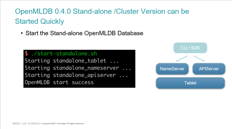
The method of using the stand-alone version is very simple. Both stand-alone version and cluster version are open-source on GitHub. The code downloaded in GitHub supports the function of cluster version at the bottom. For the stand-alone version, we provide a script. As long as this script is executed, the three components required by the stand-alone version will be started. On the right is its architecture including a Name Server service and an API Server service. The underlying data will be stored on a single Tablet, so users can access our service by using the command line or SDK.

OpenMLDB 0.4.0 Stand-alone Version to get Started Quickly | Using OpenMLDB Client

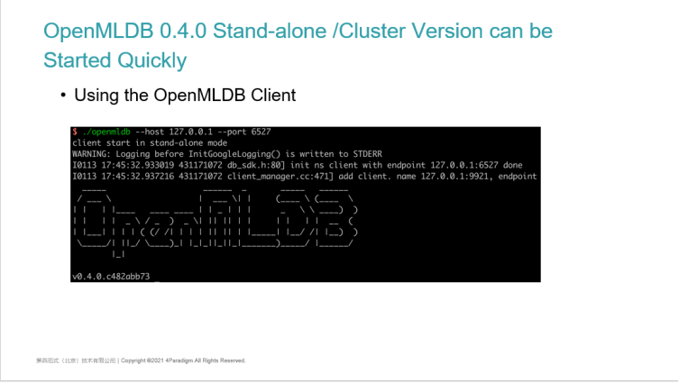
The use of the client is very simple. After starting the cluster with a script, you can use a client command-line tool like MySQL to specify the IP and port to connect to the OpenMLDB database. After connection, some basic information of the cluster will be printed including the version number and other information.

OpenMLDB 0.4.0 Stand-alone Version Quickly Get Started | Execute Standard SQL

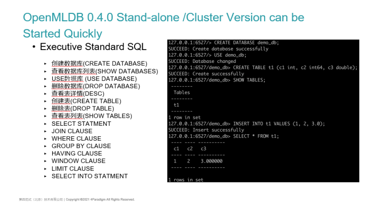
After connecting, we will be able to use the standard SQL statements.

The SQL statements we have supported are listed on the left side of the PPT. You can see a more detailed introduction in our document website. Basic SQL statements such as DML and DDL have been supported. SELECT INTO and various SELECT sub query statements can also be supported.

On the right are some screenshots of executing SQL commands. The general process of using the database is:

Create a database and a Use database. The subsequent SQL operations will be completed on the default DB
We can Create table which also follows the ANSI SQL syntax of the standard. However, compared with standard SQL, we can also specify indexes and time columns when creating tables
Through Show tables, you can see the created tables.

We also support standard SQL insert statements which insert a single piece of data into the database table and query through the select statement. This is some functions provided by the OpenMLDB as a most basic online database.

OpenMLDB 0.4.0 Cluster Version Quick Start | Start the Cluster Version of OpenMLDB Database

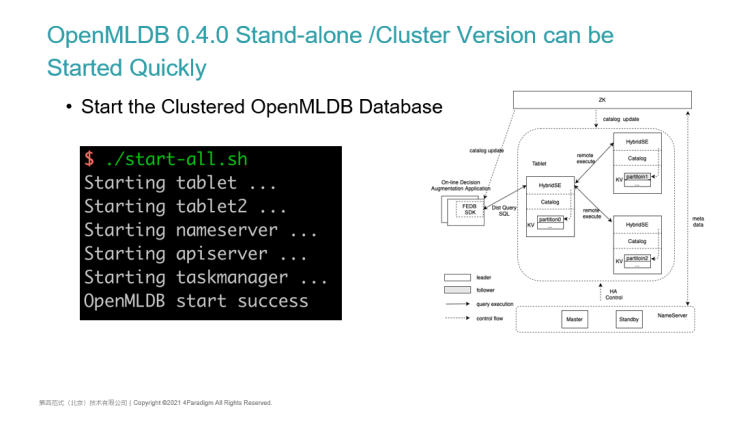
Next, I will introduce the cluster version. The start-up method of the cluster version is similar to that of the stand-alone version. We will provide a star-all script. Compared with the stand-alone version, the cluster version has the characteristics of high availability and multiple components.

First of all, there will be more components. In addition to starting the aforementioned Tablet, Name Server and the API Server, we will start two Tablets by default in order to achieve high availability, so as to ensure that all data is backed up at least twice.
Users can configure the number of data backups and the size of the cluster in the configuration file.
A very important point is that the offline task management is supported in version 0.4.0, so a highly available task management module called task manager will also be added.

On the right side of the PPT is a basic architecture diagram. In addition to OpenMLDB itself, the implementation of high availability currently depends on a Zookeeper cluster. Some basic metadata of OpenMLDB including the primary node service and the information that needs to be persisted will be stored on ZK. After the name server starts, it will register its highly available address on ZK. The Tablet will then connect to the primary Name Server through ZK, and the Name Server will then monitor the update of some metadata.

OpenMLDB 0.4.0 Cluster Version Quick Start | Cluster Version OpenMLDB Configuration File

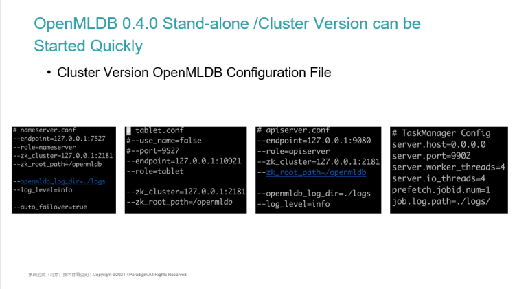
The deployment of the cluster version will be relatively complex. It adds a task manager module. You can also take a brief look at the configuration files of the technical components. The more important thing is that most components need to configure the IP and path of ZooKeep to ensure that all components are connected to the same ZooKeep. This is to realize the highly available metadata management through the Zab protocol, to ensure the high availability of the whole cluster.

OpenMLDB 0.4.0 Cluster Version Quickly Get Started | Use the Cluster Version of OpenMLDB Client

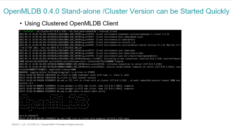
The client using the cluster version is slightly different from the stand-alone version. When using the OpenMLDB command-line client, it no longer directly specifies the IP and port of the Name Server. Because the Name Server is also highly available, its IP port may change during failover thus, we need to configure ZK information when starting. After start-up, some configuration and version information related to the cluster version will be printed.

Its use method is similar to that of the stand-alone version. We can use the SQL statements mentioned above. You can use it as an ultra-high performance, full external memory-based timing database or a database that supports SQL.

OpenMLDB 0.4.0 Cluster Version Quickly Get Started | Use the Advanced Functions of OpenMLDB in the Cluster Version

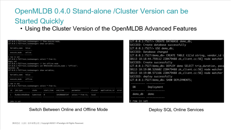
The cluster version also has some more advanced functions. Here are two:

1. Offline Mode and Online Mode. This is a unique function of the cluster version. This is because all calculations of the stand-alone version are on a stand-alone machine thus, it will not distinguish between the online mode and the offline mode. The cluster version supports the storage of massive data such as HDFS. At present, the bottom layer of the offline computing is also based on Spark.

Hence, how do you use offline mode and online mode?

We support a standard SQL Set statement whereas we can see that the current execute_mode is online. When online, the SQL statements we execute are executed through online mode. This is to check the data in the external memory.
Via set @ SESSION.exexute_mode = "offline", you can switch the mode to offline.
You can see that the current mode is offline, and the SQL query of offline mode is not to check in the external memory. This is because in the real scenario such as risk control or gang fraud identification, the offline data may be massive, ranging from a few T to hundreds of T. SQL query is certainly not interactive and can return results immediately which the query results cannot be completely aggregated on a node. Therefore, in the offline mode, we will regard SQL query as a task. You can see the basic information of the task, including task ID, task type, task status, etc.
After executing SQL, version 0.4.0 will provide some commands such as SHOW JOBS, view task status, view log information, etc., to realize this kind of offline task management. This part of the management function is also integrated into the CLI command line.

2. Deploy SQL to Online Services. This is supported by both cluster and stand-alone versions. This is not supported by other online databases. After creating the database and database tables, for a SQL that has finished feature extraction which is has been authenticated and deemed to be certified by the data scientist, you can go online through the deploy command and you can see the deployed services through the SHOW DELOPYMENT. This is a bit similar to a stored procedure in SQL. Each deployment corresponds to an online SQL. When we use online services as users, it can execute online SQL through the name of Deploy which is similar to our stored procedures.

[03 | Workshop - Fast Build a Full Online Process of the AI Application]

Finally, I will take you through a workshop to quickly start from the command line and build a full process online AI application from scratch.

Application Scenario

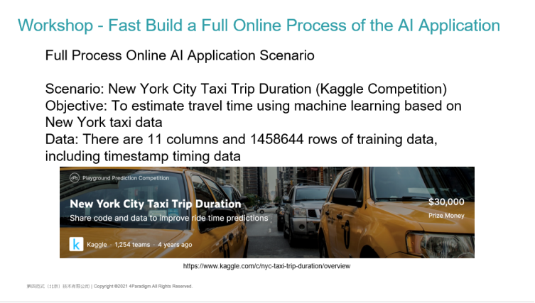
This is the scenario we demonstrated. A Kaggle Competition called the New York City Taxi Trip Duration, is a machine learning scenario for estimating travel time. We will download the historical trip data of a taxi provided by the competition. Based on these data, developers or modelling scientists need to use machine learning methods to estimate the newly given test set to estimate the trip time. The training data is not big. There are 11 columns in total which is approximately more than 1 million rows. Its feature is that it contains the timing data of the timestamp which is more important for the timing data of travel estimation scenes. We need to estimate the final travel time according to the historical records of each taxi and some characteristics of the previous sequence.

OpenMLDB 0.4.0 Technical Solution

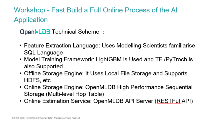
This demonstration uses the technical scheme based on OpenMLDB 0.4.0. Here is a summary:

Feature Extraction Language: The SQL language most familiar to scientific modelling scientists is used
Model Training Framework: LightGBM is used in this example. Of course, if you want to use TF or PyTorch, it can also support it
Offline Storage Engine: Use local file storage, because the data volume of its sample is not large. It has only more than 1 million lines which may be tens of megabytes of data. In the actual scene, the sample of machine learning may be larger and more complex thus, OpenMLDB can also support HDFS storage
Online Storage Engine: Using high-performance sequential storage of OpenMLDB, an external memory storage based on multi-level hop table data structure
Online Estimation Service: The API Server provided by OpenMLDB is used, and the standard Restful interface and RPC interface are provided.

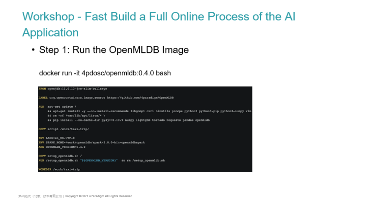
Step 1: Run the OpenMLDB Image

Next, let's demonstrate that when we use OpenMLDB for modelling. We first need to build an OpenMLDB database running environment.

OpenMLDB itself provides a test demo image. The underlying implementation of OpenMLDB is based on C++ which is relatively stable and easy to install. When using OpenMLDB, we can use the official docker image provided on GitHub. MAC environment or Linux environment can also directly download our source code, compile, and execute locally.

After execution, it will enter the container whereas the screenshot is its complete docker file content. For demo demonstration, we installed some more libraries such as pandas and Python. When you use it, you only need to install the image and Binary. You can download Binary through a script and start the server and client. The content of the image is also very clean, and there is no need to download some additional components.

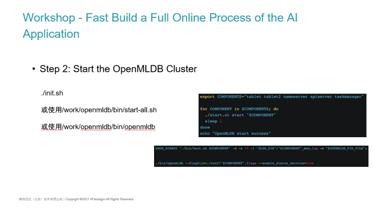
Step 2: Start the OpenMLDB Cluster

The second step is to start the OpenMLDB cluster. You can use init.sh (A script we encapsulated), or the start script provided in the OpenMLDB project which can also be started directly with the binary compiled by ourselves.

Because of the complete functions of the cluster version we demonstrate this time, we will start the zookeeper service and start some components we rely on such as Tablet, Name Server, API Server and Task Manager. As long as these components are started, we will have the function of cluster version OpenMLDB. If you are interested, you can also see the contents of the sh script. init.sh will also support stand-alone version and cluster version. When we use the cluster version, we will start an additional zookeeper and all OpenMLDB components.

In fact, the start-up of components is also very simple, which is the script content of start-all. We will define many components and make a cycle to separate each component. The start-up of these components is a Binary compiled through the OpenMLDB C++ project. Of course, different platforms should be compiled on the corresponding platform, and then use a mon tool to start it.

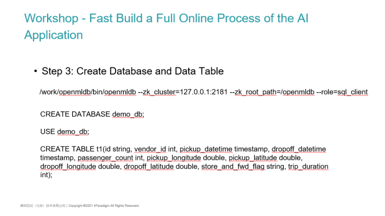
Step 3: Create Database and Data Table

After the service has been started, we can connect with a MySQL like client. As long as you configure the ZK address, you can automatically find the Name Server address and enter it into the database. At this time, you can execute most of the standard SQL statements.

To demonstrate the end-to-end machine learning modelling process of our taxi, we will:

First create a DB for testing, create database, and then use database
At this point, you can see that the database has been created through the show databases command
Then we create a table in the database. Because we haven't started the offline model training, we are unable to know what index the table needs to build in advance thus, we support users to create a table without specifying an index. Now you can see that the table has about eleven columns, and this table corresponds to the data set of the Kaggle Competition. It provides 11 column data types including multi-column timestep data.
At this point, you will be able to see the message of create successfully. The table has been created and is called T1.

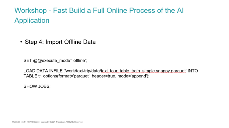
Step 4: Import Offline Data

In step 4, we need to start importing offline data and import the training data provided in the Kaggle Competition. At present, we support the import of a variety of data formats including Parquet format and CSV format.

To import offline data, we need to switch the current execution mode to offline before using the load data statement.

Why switch to offline? If you do not switch to offline, the data import at this time will become online data import. If the amount of offline data is very large, or the data is imported from HDFS, it is unreliable to import all data to our online external memory storage thus, it is very important to switch the execution mode to offline.

Then, execute an imported SQL which will submit a task. You can see the status of the task through SHOW JOBS. It is a task of importofflinedata. In a few seconds, the task has been completed and the data has been imported.

When we look at the database again, we can see that when we just imported, there was no offline data and no offline addresses. After the offline import is successful, the properties of the table will contain the offline information which indicates that the offline data has been imported to a current path. Therefore, you can see that the data file has also been imported correctly.

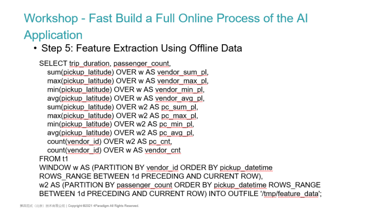
Step 5: Feature Extraction Using Offline Data

Let's continue the demonstration just now. First, switch the mode to offline. After the offline data is imported, the offline feature extraction can be carried out. This step takes different time for different modelling scenarios. Modelling scientists need to choose what features to extract, and then constantly adjust the SQL script of feature extraction.

Next, we can use the over window sliding window to do the timing characteristics to calculate its aggregate values such as min and max, or we can take the characteristics of a single line and calculate a single line for a certain line.

Finally, after the SQL is executed, we need to store the sample data after feature extraction in a location, which can be exported to a local path. If the amount of data is large, it can also be exported to an HDFS distributed storage.

At this time, you can see that the task is successfully executed. You can see that the job ID is 2 through SHOW JOBS. The job status has changed from submitted to running because it is executed in a distributed manner. Although it is not a very complex SQL, its data comes from T1 offline data. In the real offline feature extraction, the amount of data may be very large, and it is impossible to complete the SQL calculation in the local external memory thus, we will submit this task to a local or Yarn Spark for execution.

You can see that the status has changed to finished, indicating that the data has been exported successfully. The export path was specified in our SQL statement just now. We can see that the sample data has been exported correctly on the command line. In order to support more training frameworks, in addition to the CSV format supported by default, other sample formats are also supported. The content of this data file is the sample data generated through the SQL statement just now,

Step 6: Use Sample Data for Model Training

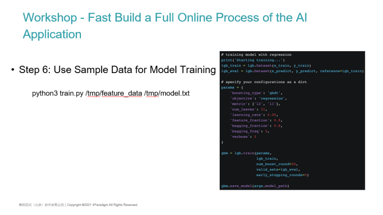
This sample data can be trained using the open-source machine learning framework. Here we use our train script. You can also take a brief look at its content. First, it introduces the LightGBM third-party library. Infront, you need to enter the path of the feature file just specified and the path of the model it needs to export.

Then, the first step is to integrate the sample data, integrate multiple CSV files into a single CSV file, and then read out the characteristics of CSV through panda. The following is a machine learning modelling script familiar to modelling users:

The first is to split the training set and prediction set of the sample and extract its label column
Transfer the Python dataset and configure the machine learning model we use such as GBDT, decision tree and DNN model
Use the train function of LightGBM to start training.

This script can also be replaced with the training script of any open-source machine learning framework such as TensorFlow, PyTorch or OneFlow. We execute this script because it doesn't have a lot of sample data, so it will soon train the new model and export it to the output path. Later, we can use this model to launch the model. However, we must consider that our model online is not just the influence of the model. Our input data is the original data provided by Kaggle. All end-to-end machine learning processes must include feature extraction and the influence of the model.

Step 7: Deploy SQL Online

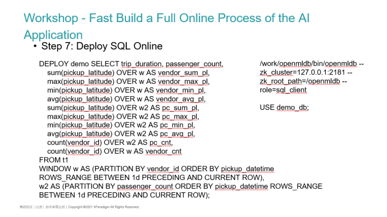
We need to use a high-performance online feature engineering function provided by OpenMLDB to put the SQL just modelled online. We re-enter the OpenMLDB database from the client and switch its default DB. The SQL deployment is the same as the previous SQL offline feature engineering. Currently, we don't need to make special development for a feature. We just need to use the same SQL statement and add the deploy statement in front to make SQL Online. During deploy, it will partition some keys and sort the time columns. We will index these keys in advance and arrange and store these data according to the index.

Step 8: Import Online Data to OpenMLDB

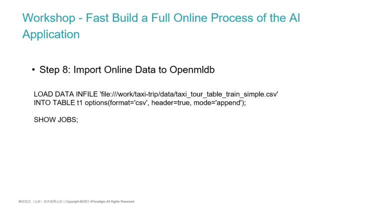
After the deployment, we can make online estimation. During the estimation, we certainly hope to realize online estimation. This is because the feature we do is this time-series window feature. We hope that when calculating each feature, we can aggregate min or max according to the window of the previous day thus, we generally carry out a water storage operation. This is to import some online data into the online database. Online import is also a distributed task. After execution, we can see that a job has been submitted, and the job is running very fast. In the local environment, its performance is very good. We can see that job3 has been completed and the data has been imported.

Step 9: Start HTTP Estimation Service and Online Estimation

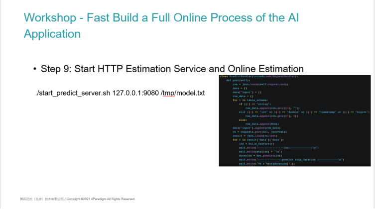
With the imported online data, we can start the estimation service to make online estimation in step 9. The estimation service is packaged. There is a script called start predict server. This script is a very simple Python HTTP server encapsulated by us. The HTTP server will wrap some client data requests to the API Server, and finally print the results. After the original data comes in, the sample data is obtained through feature engineering, and the LightGBM model just obtained from model training will be loaded. The model should be used to receive the feature samples returned online, and then the prediction results will be returned.

Step 10: Online Feature Extraction Calculation

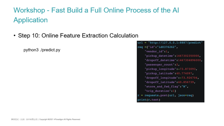
We start the predict server first, and the last step is to do online predict.

Online predict is a script encapsulated by us. This script is an HTTP client. It will pass in the original data column provided by us (these inputs include string type data, not the sample after feature extraction) as parameters and execute it directly through Python. It can be executed quickly. A single online feature extraction can be done within 10 milliseconds.

How is this speed achieved? This is related to the SQL complexity of our user modelling. For simple features like this, if the amount of data is relatively small, it can even be achieved within 1 millisecond. With the time of pure feature engineering and the time estimated by the model, the user returns immediately without any perception. Here are the online samples of feature samples made through our SQL statements, and then this is the data estimated by a model returned by LightGBM.

Some people may think that running a few scripts seems to be nothing. You just do some SQL calculations. I go to MYSQL to check the data. It seems that it can also return within tens of milliseconds or 100 milliseconds. What's the difference?

Like the feature store mentioned by the audience just now, it can also support this feature storage, and then it can also support simple feature engineering. For example, you can pass a feature, trip_duration may be 10, and then your feature is to normalize it or transform it. In fact, this feature is a single line feature. Obviously, the performance of single line feature is very high. Whether it is implemented in Python or C++, you need almost only one CPU calculation to multiply and add an original data.
The feature we support is actually the timing aggregation feature of a sliding window. When calculating the data of an input line, the calculation is not only a numerical calculation for this line. You need to take out all the data of this line before the day from the database, and then define the syntax according to the window of ROW BETWEEN or RANGE BETWEEN, slide the window, and then aggregate the data in the window. Our performance within 10 milliseconds is the result of different aggregation for these two features.
If we don't use a special time series database, for example, we obtain all the data of the previous day of its current row data from MySQL, the window data acquisition may take more than 100 milliseconds. We can achieve window data acquisition, window feature aggregation and final model estimation, and the overall time can be controlled within 10 milliseconds to 20 milliseconds. This is closely related to our storage architecture design, and it is also the difference between our OpenMLDB and other OLTP databases. Finally, we can get an estimated result.

Summary of AI Application in the Full Process of Launch

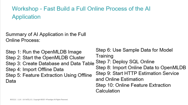
Let's summarize the 10 steps of the online full process AI application. In fact, the previous steps are relatively simple. They are start the OpenMLDB cluster, Create a Database, Create a Table, and then Import Offline Data and Calculate Offline Characteristics. When the SQL of feature extraction have no issue, we can launch the SQL. After launching, we will start a prediction service that supports HTTP, and then make a prediction. In version 0.4.0, almost all steps can be executed and supported on the command line of SQL. In the future, we also plan to support online feature extraction based on the command line, and even expand SQL syntax on the command line to support model training on the command line.

Finally, a brief summary of this sharing will be given. First, we will introduce some new features of the whole process of OpenMLDB 0.4.0, as well as the rapid start of stand-alone and cluster versions. In the end, we will demonstrate how to use OpenMLDB to fast build an AI application that can go online through a Kaggle Competition scenario.

Welcome to our community. At present, all the documents and codes of the project are on GitHub. If you are interested, you can also participate in the submission of issue and the development of pull request code. Welcome to join our WeChat communication group by scanning your code. That's the end for my sharing. Thank you very much for listening.